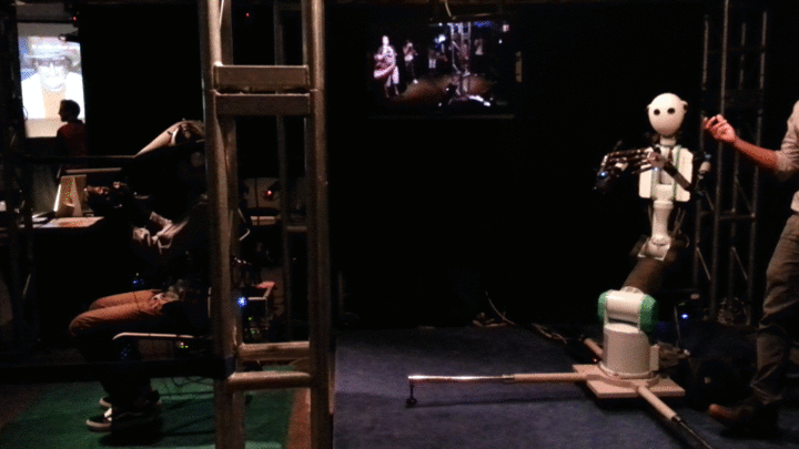
Low-noise Stills from Video
Supasorn Suwajanakorn / Andre Baixo
Introduction
Goals
Related work
- Video Snapshots: Creating High-Quality Images from Video Clips. by K. Sunkavalli, N. Johsi, Sing Bing Kang, M.F.Cohen, H. Pfister, is a unified framework for generating a single high-quality still image ("snapshot”) from a short video clip. Their system allows the user to specify the desired operations for creating the output image, such as super resolution, noise and blur reduction, and selection of best focus. It also provides a visual summary of activity in the video by incorporating saliency-based objectives in the snapshot formation process.
- A High-Quality Video Denoising Algorithm based on Reliable Motion Estimation. by Ce Liu, William T. Freeman, proposes an adaptive video denosing framework that integrates robust optical flow into a non-local means (NLM) framework with noise level estimation. In addition, they use approximate K-nearest neighbor matching to significantly reduce the complexity of classical NLM methods.
- Efficient video denoising based on dynamic nonlocal means by Y. Han, R. Chen is based on dynamic nonlocal means (DNLM) under the Kalman filtering framework. However, their DNLM is not competitive with several state-of-the-art video denoising algorithms.
Algorithm

The first frame in the video sequence will be used as a reference frame for which we try to reduce the noise. On the reference frame, we detect features using SURF feature detector, then we track those feature points throughout the video sequence using Lucas-Kanade tracking method. These tracked features will provide sparse correspondences between each frame and the reference. We perspective-warp each frame to the reference by robustly solving for a 3 x 3 homography via RANSAC. Then we run polynomial expansion-based Farneback's optical flow algorithm between each frame and the reference which is fast and gives low interpolation error but has high endpoint and angular errors. The two latter errors however are not important in our task because we only care about image similarity. Suppose these aligned frames are $I^1, I^2, \dots, I^n$ and $I^0$ is the reference, we compute $D^i = G * (I^0 - I^i)$ where $G$ is a truncated Gaussian kernel of size 3 x 3 and $*$ is the convolution operator. Then we weight the contribution from each pixel in each frame based on color similarity. A noise-reduction version of $I^0$ is given by:
$Z$ is the normalization factor and $D^i_{uv}$ is a vector that encodes RGB values for pixel $uv$. $\sigma$ controls the similarity weight.
This similarity-based weight can handle small scene motions, but for large motions, there can be cases where the average pixels are close to those of $I^0$ but represent different objects such as when the exact pose of a person in the reference frame, for example, appears in only a few frames and the average converges to a different value but close to the true value. In such case, it is sometimes more desirable to retain the noisy original pixels. One way to solve this problem is to apply a threshold to the color difference and retain original pixels when the sum is too large. Again, to make the algorithm more robust against noise, the sum of color differences around a Gaussian patch is used instead. (Assuming zero-mean noise, the sum of differences around the same patch should be close to zero.) This threshold alone can cause noisy artifacts, so we simply enforce spatial smoothness using Markov random field defined on a standard 4-connected grid. The label set is $\{0, 1\}$ where 0 means the original pixels should be used and 1 means the computed average should be used. The energy functional decomposes into a dataterm $\phi$ and a smoothness term $\psi$:
We encode the color theshold into the dataterm as follows:
A hard threshold on $D^i_{uv}$ can be achieved by using some appropriate set of $\alpha, \beta_0, \beta_1$. The smoothness term is only non-zero when $\psi(x_i, x_j \neq x_i) = \gamma$ which penalizes different adjacent labels. This binary segmentation problem is solved using graph-cut which gives us a global-optimal labeling $X: \mathbb{R}^d \rightarrow \{0,1\}$. We then erode this labeling function and apply Gaussian blur to transform 0-1 labeling into a continuous alpha mask. The final low-noise composite is computed using a simple interpolation $(1-x_i)I^0 + x_i\widetilde{I^0}$.
Experiments
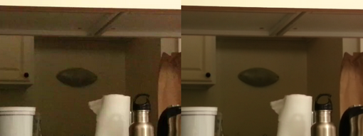
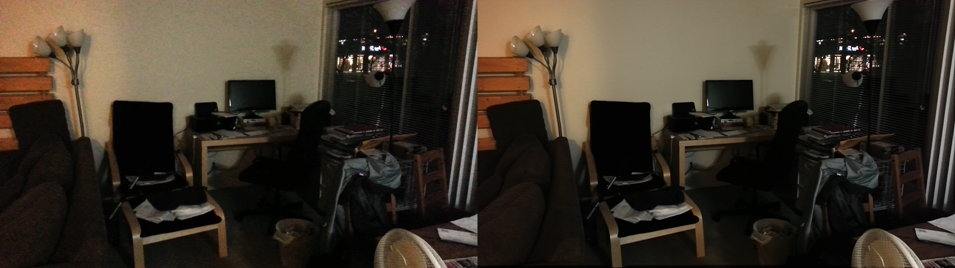
Left: cropped input. Right: cropped output using dense optical flow
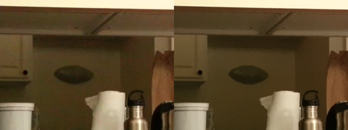
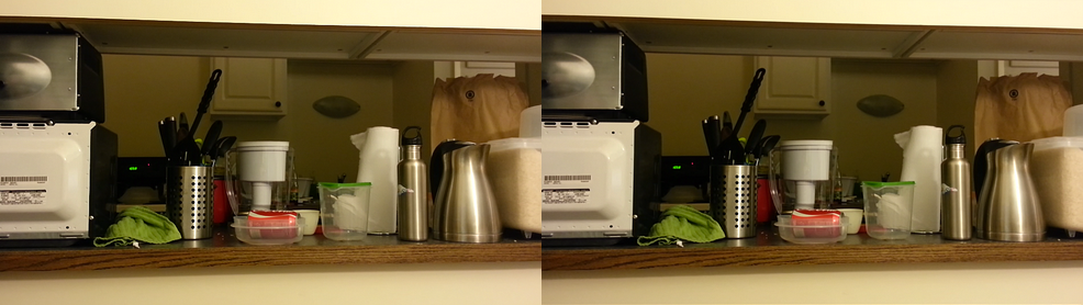
Left: cropped input. Right: cropped output using bilateral filtering
We discovered Farneback's algorithm based on polynomial expansion which runs very fast (less than a second) compared to a variational approach (100 seconds), but it cannot handle large motions and the flow seems to be inaccurate around the untextured regions.
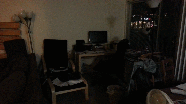
Two frames that we test two optical flow algorithms on.
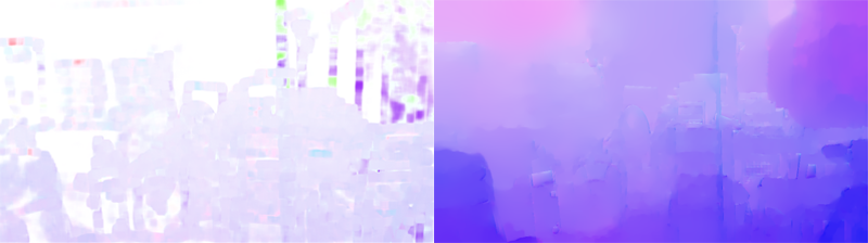
Left: color-coded flow field from Farneback's algorithm. Right: flow field from Ce Liu's implementation. Notice that the flow field from Farneback's algorithm isn't propagated correctly to untextured regions.
In order to handle larger motions with Farneback's algorithm, we therefore perform a global alignment using homography before running the dense optical flow as in our current pipeline. This hugely improves the alignment quality as shown below.

Left shows Farneback's warps without doing global alignment first. Right shows warps with global alignment which appears almost identical to the left image.
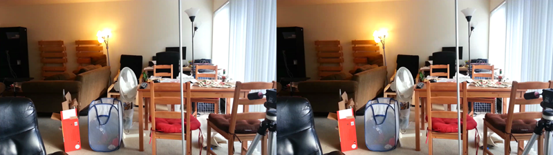
When we compare our results that use fast Farneback's optical flow to ones that use variational approach, the quality does not visually degrade on many datasets that we tried while running orders of magnitude faster.
Left shows a result from variational optical flow. Right shows a result with Farneback's optical flow + global alignment.
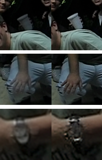
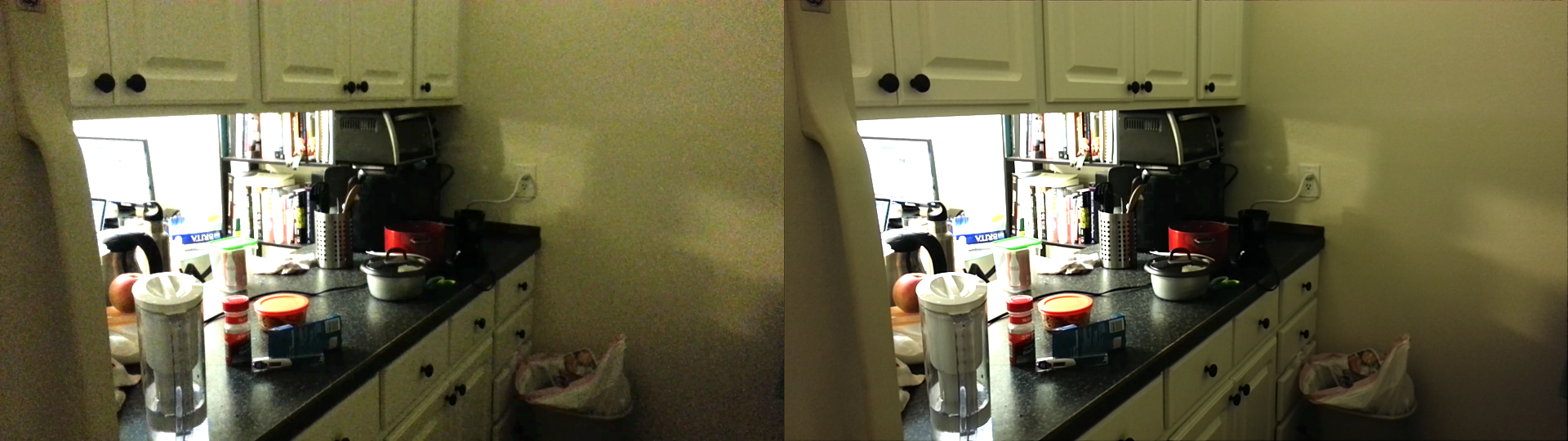
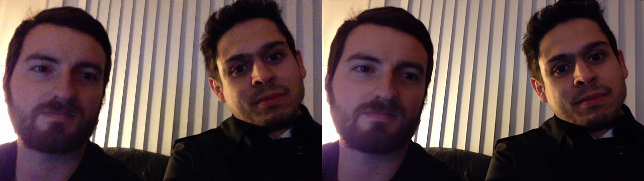
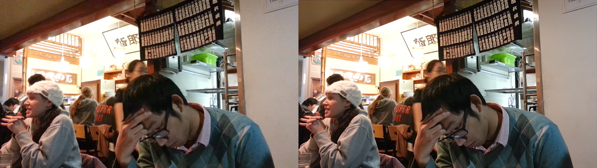
Photos on the left are examples of ghosting artifacts and photos on the right are results using similarity-based averaging.
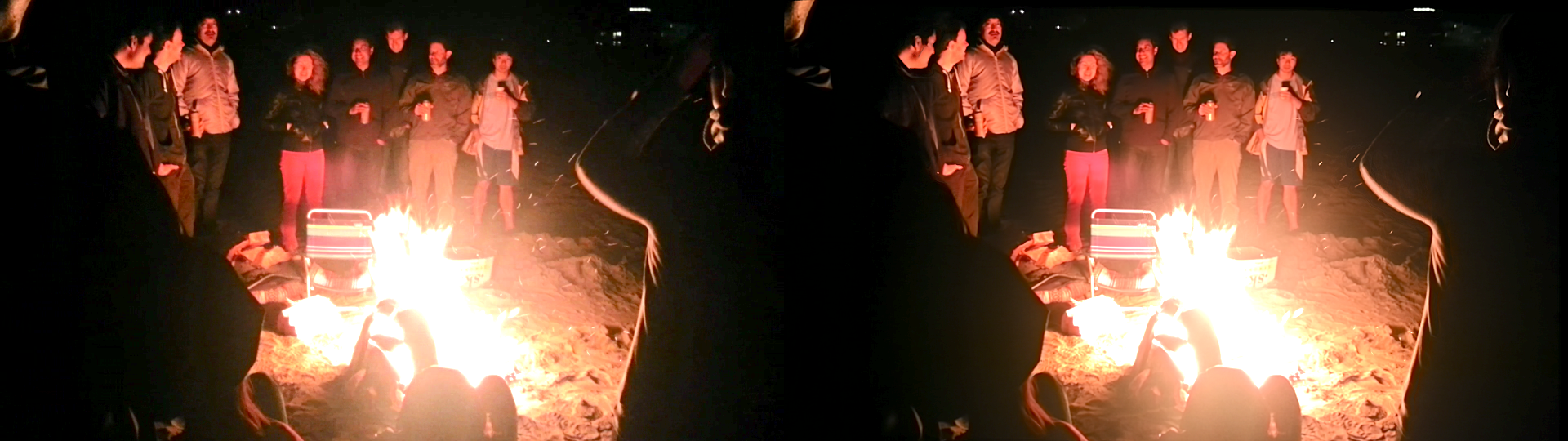
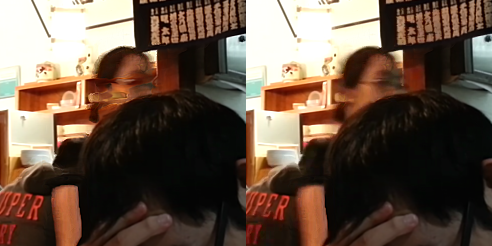
However, when the video clip contains large movements and there are no other frames that have similar scene appearance to the reference frame, the similarity-based weights can produce another kind of artifacts shown below.
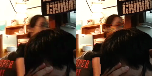
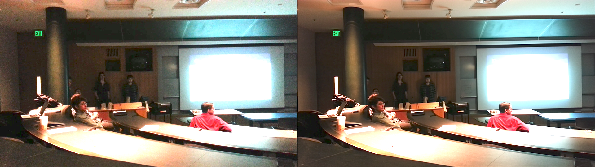
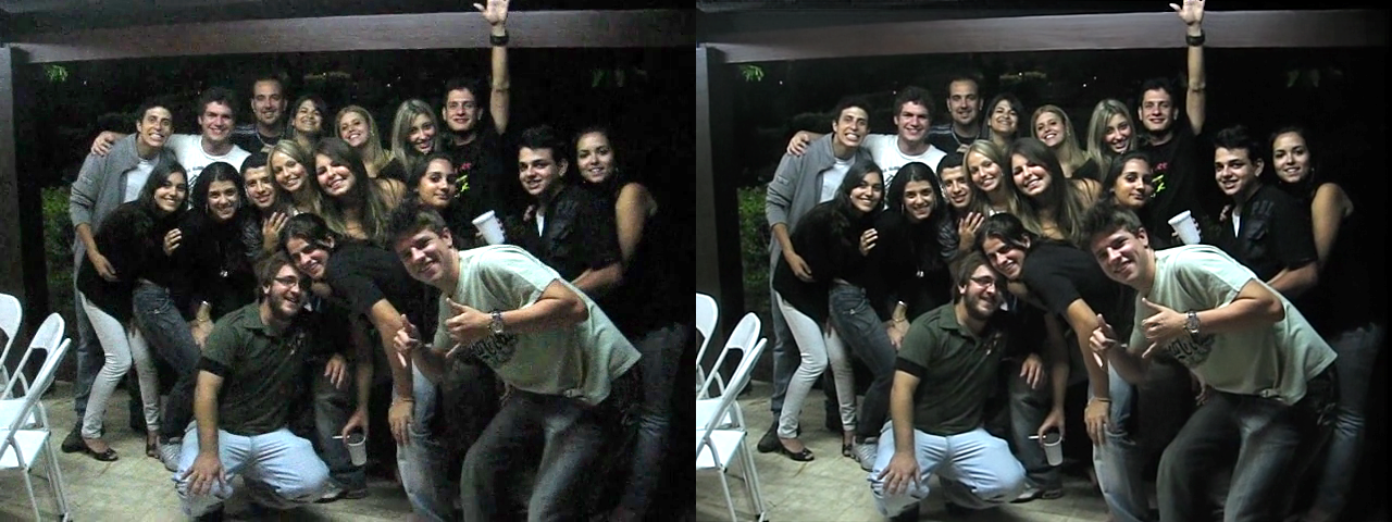
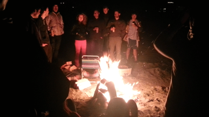
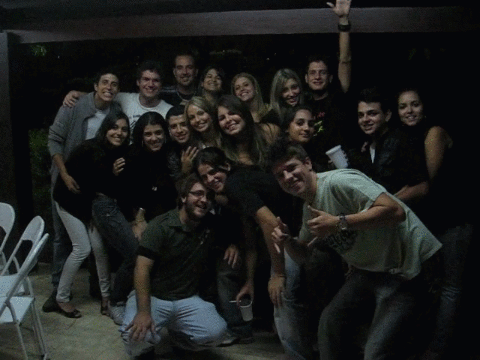
Top shows the input video sequence. Bottom left shows the reference frame and bottom right shows a result from similarity-based averaging.
We overcome this problem by applying threshold on color difference and retain the original pixel when the difference is too high. Together with smoothness term in MRF, we are able to handle pixels that appear a few times or once in the reference frame without producing the above artifacts or ghosting.
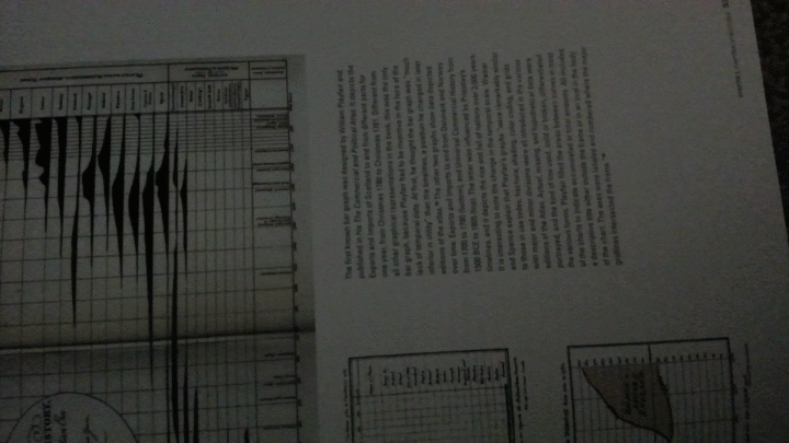
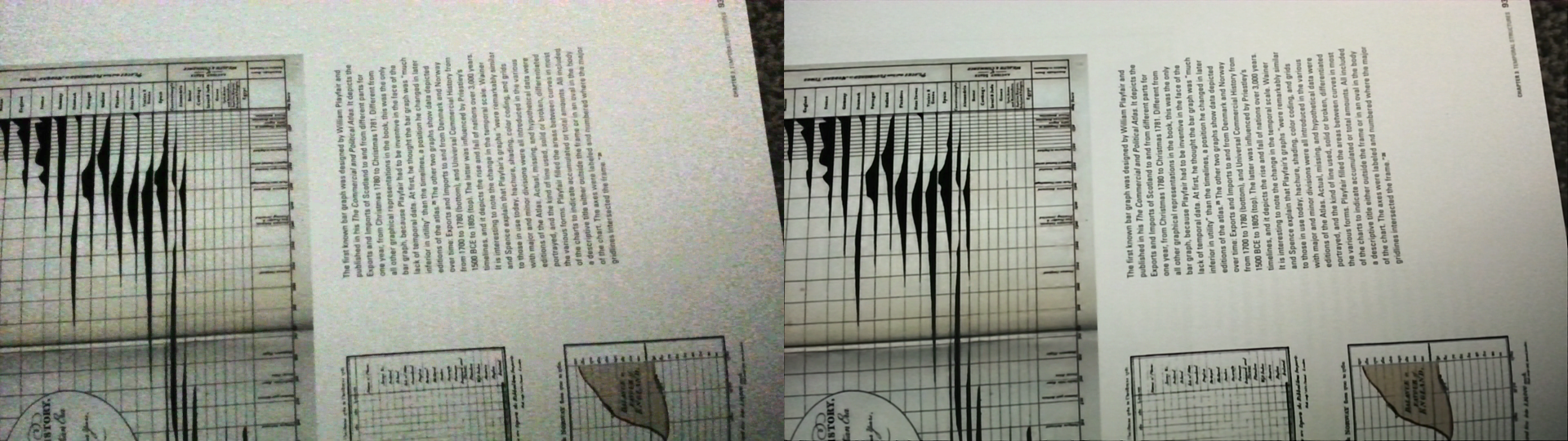
Comparing results without MRF on the left and with MRF and thresholding on the right.